The Fibonacci series is a sequence of numbers where each number is the sum of the two preceding ones, usually starting with 0 and 1. It has significant importance in computer science and mathematics, appearing in various algorithms and data structures. This article will delve into how to implement a Fibonacci series program in Ruby, covering multiple approaches such as iterative, recursive, and memoized methods. We will also explore the mathematical properties of the Fibonacci sequence and its applications.
Basic Array Operations in Ruby
Understanding the Fibonacci Series
The Fibonacci sequence is defined as follows:
F(0) = 0
F(1) = 1
F(n) = F(n-1) + F(n-2) for n > 1
The first few numbers in the Fibonacci sequence are:
0, 1, 1, 2, 3, 5, 8, 13, 21, 34, ...Each number is the sum of the two preceding numbers. This sequence grows exponentially and finds applications in areas such as computer algorithms, financial models, and biological settings.
Iterative Approach
The iterative approach to generating Fibonacci numbers is straightforward. It uses a loop to calculate each Fibonacci number up to the desired position.
Example: Iterative Fibonacci Series
def fibonacci_iterative(n)
  return n if n <= 1

  fib_0 = 0
  fib_1 = 1

  (2..n).each do
    fib_n = fib_0 + fib_1
    fib_0 = fib_1
    fib_1 = fib_n
  end

  fib_1
end

# Example usage
n = 10
puts "The #{n}th Fibonacci number is: #{fibonacci_iterative(n)}"
Explanation
- Base Case: If
nis 0 or 1, the function returnsndirectly. - Loop: The loop starts from 2 and continues to
n, updating the values offib_0andfib_1to store the two most recent Fibonacci numbers. - Return: After the loop,
fib_1holds thenth Fibonacci number.
Recursive Approach
The recursive approach directly follows the mathematical definition of the Fibonacci series. This method is elegant but can be inefficient for large n due to repeated calculations.
Example: Recursive Fibonacci Series
def fibonacci_recursive(n)
  return n if n <= 1
  fibonacci_recursive(n - 1) + fibonacci_recursive(n - 2)
end

# Example usage
n = 10
puts "The #{n}th Fibonacci number is: #{fibonacci_recursive(n)}"
Explanation
- Base Case: If
nis 0 or 1, the function returnsn. - Recursive Call: For other values of
n, the function calls itself to calculatefibonacci_recursive(n - 1)andfibonacci_recursive(n - 2)and returns their sum.
Performance Considerations
While the recursive approach is simple, it has exponential time complexity (O(2^n)) because it recalculates Fibonacci numbers multiple times. For large n, this can lead to significant inefficiencies.
Memoization Approach
To optimize the recursive approach, we can use memoization. Memoization stores previously calculated Fibonacci numbers to avoid redundant calculations, improving performance significantly.
Example: Memoized Fibonacci Series
def fibonacci_memoized(n, memo = {})
  return n if n <= 1

  unless memo.key?(n)
    memo[n] = fibonacci_memoized(n - 1, memo) + fibonacci_memoized(n - 2, memo)
  end

  memo[n]
end

# Example usage
n = 10
puts "The #{n}th Fibonacci number is: #{fibonacci_memoized(n)}"
Explanation
- Base Case: If
nis 0 or 1, the function returnsn. - Memoization Check: Before making recursive calls, the function checks if the result for
nis already stored inmemo. If not, it calculates and stores the result. - Return: The function returns the memoized result.
Performance Improvement
The memoized approach has a time complexity of (O(n)) and space complexity of (O(n)), making it much more efficient than the naive recursive approach for large n.
Dynamic Programming Approach
The dynamic programming approach builds the Fibonacci series from the bottom up, storing intermediate results in an array. This method is both time-efficient and space-efficient.
Example: Dynamic Programming Fibonacci Series
def fibonacci_dp(n)
  return n if n <= 1

  fib = Array.new(n + 1)
  fib[0] = 0
  fib[1] = 1

  (2..n).each do |i|
    fib[i] = fib[i - 1] + fib[i - 2]
  end

  fib[n]
end

# Example usage
n = 10
puts "The #{n}th Fibonacci number is: #{fibonacci_dp(n)}"
Explanation
- Initialization: An array
fibis created withn+1elements, withfib[0]andfib[1]initialized to 0 and 1, respectively. - Loop: The loop calculates each Fibonacci number from 2 to
n, storing the results in thefibarray. - Return: The function returns the
nth Fibonacci number stored infib[n].
Performance
This approach has a time complexity of (O(n)) and space complexity of (O(n)). However, space complexity can be optimized to (O(1)) by storing only the last two Fibonacci numbers instead of the entire array.
Optimized Dynamic Programming Example
def fibonacci_optimized(n)
  return n if n <= 1

  fib_0 = 0
  fib_1 = 1

  (2..n).each do
    fib_n = fib_0 + fib_1
    fib_0 = fib_1
    fib_1 = fib_n
  end

  fib_1
end

# Example usage
n = 10
puts "The #{n}th Fibonacci number is: #{fibonacci_optimized(n)}"
Mathematical Approach
The Fibonacci sequence can also be calculated using a closed-form expression known as Binet’s formula. Although it involves floating-point arithmetic and is less common in practical programming, it provides an interesting mathematical perspective.
Binet’s Formula
F(n) = (φ^n - ψ^n) / √5where
- φ (phi) = (1 + √5) / 2
- ψ (psi) = (1 – √5) / 2
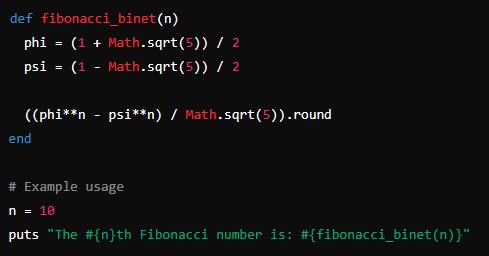
Example: Fibonacci Using Binet’s Formula
def fibonacci_binet(n)
  phi = (1 + Math.sqrt(5)) / 2
  psi = (1 - Math.sqrt(5)) / 2

  ((phi**n - psi**n) / Math.sqrt(5)).round
end

# Example usage
n = 10
puts "The #{n}th Fibonacci number is: #{fibonacci_binet(n)}"
Explanation
- Constants:
phiandpsiare calculated using the square root of 5. - Formula Application: The formula
(phi**n - psi**n) / Math.sqrt(5)is applied and the result is rounded to the nearest integer.
Performance Considerations
While Binet’s formula is mathematically elegant, it is not commonly used in programming due to potential inaccuracies with floating-point arithmetic, especially for large n.
Applications of Fibonacci Series
The Fibonacci sequence has numerous applications in computer science, mathematics, and nature. Some notable examples include:
Computer Science
- Algorithm Design: Fibonacci numbers are used in various algorithms, such as dynamic programming and divide-and-conquer strategies.
- Data Structures: Fibonacci heaps, a type of priority queue, use Fibonacci numbers to achieve efficient performance.
- Search Algorithms: Fibonacci search is an efficient searching algorithm for sorted arrays.
Mathematics
- Number Theory: Fibonacci numbers have unique properties and relationships with other number sequences, such as Lucas numbers and the golden ratio.
- Combinatorics: Fibonacci numbers appear in combinatorial problems, such as counting paths on a grid or tiling problems.
Nature
- Biological Settings: Fibonacci numbers are observed in the branching patterns of trees, the arrangement of leaves, the fruit sprouts of a pineapple, and the flowering of artichoke.
- Growth Patterns: The sequence describes idealized population growth in certain animal species, such as rabbits.
Conclusion
The Fibonacci series is a fascinating and fundamental concept in both mathematics and computer science. In Ruby, there are multiple ways to implement a Fibonacci series program, each with its own advantages and trade-offs. From the simple iterative approach to the more advanced memoization and dynamic programming techniques, understanding these methods will enhance your problem-solving skills and deepen your appreciation for the beauty of the Fibonacci sequence. Whether you are interested in algorithm design, data structures, or exploring mathematical properties, mastering the Fibonacci series is an essential step in your programming journey.